
 ACCESS
Research Article
ACCESS
Research Article
Volume 2, Article ID: 2025.0010

Tianming Zhu
tianming.zhu@nie.edu.sg


Carol Anne Hargreaves
carol.hargreaves@nus.edu.sg

Yi Xin Cheng

Christopher Chen Li-Hsian
phccclh@nus.edu.sg
Siama Hilal
1 National Institute of Education, Nanyang Technological University, Singapore 637616, Singapore
2 Department of Statistics and Data Science, National University of Singapore, Singapore 117456, Singapore
3 Department of Pharmacology, Yong Loo Lin School of Medicine, National University of Singapore, Singapore 117600, Singapore
4 Saw Swee Hock School of Public Health, National University of Singapore, Singapore 117549, Singapore
* Author to whom correspondence should be addressed
Received: 02 Jan 2025 Accepted: 28 Jan 2025 Available Online: 15 Jan 2025 Published: 20 Mar 2025
Dementia is a decline in cognitive function, typically diagnosed when the acquired impairment becomes severe enough to impact social or occupational functioning. Between no cognitive impairment (NCI) and dementia, there are many intermediate states. Predictive cognitive impairment can be useful for initiating treatment to prevent further brain damage. Several deep learning-based approaches have been proposed for the classification of Magnetic Resonance Imaging (MRI) to diagnose Alzheimer’s disease (AD) or dementia. However, diagnoses of cognitive impairment are not based solely on MRI data but also on other associated factors. In this study, the aim is to predict cognitive impairment using both neuroimaging markers and other associated factors, employing a deep learning autoencoder algorithm based on data from a Singapore study. A novel method has been proposed for applying autoencoders to a multiclass classification task and provide a feature importance analysis. The performance of the autoencoder model was compared with two widely used machine learning classification algorithms, namely, the multinomial logistic regression (MLR) and Extreme Gradient Boosting (XGBoost). The results show that the autoencoder algorithm performs well and outperforms the competing methods.
Dementia and cognitive impairment represent a significant public health challenge worldwide [1]. According to the Alzheimer’s Association International Conference (AAIC) 2021, an estimated 10 out of every 100,000 individuals develop early-onset dementia (before age 65) each year, amounting to 350,000 new cases annually across the globe. In 2019, Alzheimer’s disease (AD) and other forms of dementia were ranked as the 7th leading cause of death, based on the World Health Organization’s report on the top 10 causes of death [2]. Dementia is typically chronic or progressive, often beginning with a cognitively normal stage or no cognitive impairment (NCI), advancing to mild cognitive impairment (MCI), and eventually leading to AD [3]. Early detection and accurate prognosis of this devastating disease are complex due to its heterogeneous mechanisms. Deep-learning approaches have recently gained traction in healthcare, with significant applications proposed for classifying neuroimaging data associated with Alzheimer’s disease (AD) and other forms of dementia. Convolutional Neural Network (CNN) first gained prominence in 2012 by achieving state-of-the-art performance on the ImageNet Large-Scale Visual Recognition Challenge (ILSVRC) [4]. Since then, CNNs have become the most widely used technique for MRI datasets. In [5], a CNN was trained from scratch for early detection of AD. Additionally, [6] developed the DEMentia NETwork (DEMNET) model based on CNN, which was trained and tested on various datasets to detect different stages of dementia from MRI and address the issue of class imbalance. In [7], AlzeimerNet was introduced, a fine-tuned CNN classifier capable of identifying five stages of AD. Moreover, a deep residual neural network combined with other transfer learning techniques was trained in [8] for categorizing AD. Lately, [9] proposed an unsupervised convolutional autoencoder network for classifying AD and normal controls. [10] presented a method for classifying or distinguishing AD using a support vector machine (SVM) combined with a feature selection technique. [11] employed a machine learning model integrated with an artificial neural network (ANN) algorithm to predict cognitive impairment based on the neuropsychological test data. In [12], a combined approach of machine learning and semi-parametric survival analysis was used to estimate the relative importance of 52 predictors in forecasting cognitive impairment and dementia within a large, population-representative sample of older adults. [13] proposed a multitask weakly-supervised attention network (MWAN) for the joint regression of multiple clinical scores from baseline MRI scans. [14] introduced a novel DCGAN-based Augmentation and Classification (D-BAC) model approach for identifying and classifying dementia into various categories based on MRI scan prominence and severity. Finally, [15] conducted a comprehensive comparative study of various generative pipelines including Generative Adversarial Networks (GANs), Variational Autoencoders, and Diffusion Models, to address data scarcity and related challenges. Generally, deep neural networks have demonstrated performance equal to or surpassing that of clinicians in many tasks, due to the rapid growth in available data and computational power. In this paper, we aim to develop deep learning algorithms for classifying cognitive impairment using a process similar to clinician diagnoses. Clinicians diagnose cognitive impairment or dementia not only by evaluating MRI but also by considering other associated risk factors such as demographic information and cardiovascular health. Therefore, in this study, the aim is to classify cognitive impairment based on both neuroimaging markers and associated risk factors. To the best of our knowledge, this approach is novel in the field of cognitive impairment classification. The primary deep learning algorithm used in this study is the autoencoder which was first introduced in [16]. An autoencoder is an unsupervised ANN algorithm that aims to produce output identical to its input. Its architecture consists of two main components: the encoder and decoder. The encoder compresses the input data into a lower-dimensional space, known as the latent space. The compressed data is then passed to the decoder, which reconstructs the original data. Ideally, the output of the decoder (the reconstructed data) should closely match the input data. The difference between the input data and reconstructed data is called reconstruction error. A smaller reconstruction error indicates a higher similarity between the reconstructed data and original data. Autoencoder is commonly used for anomaly detection and have been shown to perform well in detecting anomalies in brain MRI (see [17] for more details). For anomaly detection, the autoencoder is typically trained using normal data only. For a new observation, if the reconstruction error exceeds a threshold, it is called an anomaly. However, determining this threshold is challenging and can be subjective. To address this issue, we propose a novel approach using an autoencoder that can handle classification problems without requiring a predefined threshold. The main contributions of this study are as follows. First, we developed an innovative method that extends the use of the autoencoder beyond traditional unsupervised tasks to include multiclass classification, enabling the identification of intermediate cognitive impairment states rather than limiting the analysis to a binary classification of dementia. This advancement expands the autoencoder’s capabilities and enhances its utility across various domains. The method tackles the significant challenge of determining an appropriate threshold for the reconstruction error, a common issue when using autoencoders for anomaly detection. The classification results, demonstrate the effectiveness of our proposed approach in handling multiclass classification tasks. Secondly, this work is based on a Singapore study, where the subjects were drawn from a population-based cohort. Unlike previous studies, both neuroimaging markers and various risk factors were considered in the analysis. By incorporating demographic and cardiovascular risk factors alongside MRI data, our approach mirrors more closely the clinical diagnosis process for cognitive impairments in real-life scenarios. Finally, we propose a method for obtaining feature importance analysis from this autoencoder-based classifier. The important features identified by our method are consistent with those derived from existing classifiers. The rest of the paper is organized as follows. Section 2 gives a brief overview of demographic information, risk factors, neuroimage markers and exploratory data analysis of the dataset used in this study. Section 3 details the methods and experiments applied in this study, in particular, the application of the autoencoder algorithm for multiclass classification problems and the method for obtaining feature importance is outlined. The classification results are given in Section 4 and the conclusions and future work are presented in Section 5.
2.1. Overview This study was conducted using the data from the Epidemiology of Dementia in Singapore (EDIS) study. Participants, aged 60–90 years, were drawn from the Singapore Epidemiology of Eye Disease (SEED) study, a population-based study involving Chinese (Singapore Chinese Eye Study [SCES], [18]), Malays (Singapore Malay Eye Study [SiMES-2], [19]), and Indians (Singapore Indian Eye Study [SINDI-2], [20]). The dataset contains n = 864 subjects with p = 67 variables, including subject ID, diagnosis, demographic information, risk factors, neuroimaging markers and assessment scores used for evaluating cognitive impairment and dementia. Cognitive Impairment No Dementia (CIND) was defined as impairment in at least one domain of a neuropsychological test battery (NTB), which assesses seven domains, including five non-memory and two memory domains. CIND mild was diagnosed when no more than two domains were impaired, while CIND moderate was diagnosed when more than two domains were impaired. For more details, see [18] and [21]. Thus, the subjects can be categorized into four classes based on their diagnosis of cognitive impairment and dementia, namely, NCI, CIND mild, CIND moderate, and Dementia. Since the test scores were used for diagnosing cognitive impairment, they were excluded from the prediction models. As a result, we manually selected p = 25 variables for this study. Further, the observations were removed with missing values and potential outliers. For each class, values beyond three standard deviations from the mean were considered outliers, and observations containing outliers were removed. As a result, 78 observations were excluded from the dataset. The cleaned dataset comprises n = 786 observations: n1 = 238 with NCI, n2 = 258 with CIND mild, n3 = 263 with CIND moderate, and n4 = 27 with Dementia. Due to the low number of dementia cases, as suggested by the clinicians, CIND moderate and Dementia were combined into a single category for classification analyses, referred to as the CIND moderate/Dementia group. The exploratory data analysis involved grouping the variables into three clusters, namely, basic demographic information, risk factors, and neuroimaging markers. For categorical variables, the contingency table was displayed, and Pearson’s chi-squared test was conducted to determine whether the distribution of counts for those diagnosed with and without cognitive impairment differs. For continues variables, we plotted boxplots and performed pairwise Student’s t-test [22] to assess whether the means for different groups are significantly different. The detailed results of the exploratory data analysis for these three clusters are presented in the following subsections. Note that the prevalence of any cognitive impairment was calculated as (n2 + n3 + n4)/n, representing the proportion of subjects with either CIND mild, CIND moderate, or Dementia. 2.2. Basic Demographic Information This subsection includes basic demographic information about the subjects, such as age, race, gender, and education level. For age, we categorized the continuous variable into three groups, namely, 60–69 years, 70–79 years, and 80 years and older. There are 396 individuals aged between 60–69, 315 aged between 70–79, and 75 aged 80 and above. The prevalence of any cognitive impairment (in %) for each feature is displayed in Table 1 below. Demographic information. From Table 1, several conclusions can be drawn. Firstly, adults over 80 years of age have the highest prevalence of cognitive impairment at 97.33%, followed by those aged 70–79 years at 79.68%, and those aged 60–69 years at 56.57%. As age increases, the prevalence of any cognitive impairment increases. Secondly, the Chinese have the lowest prevalence of cognitive impairment at 57.20%, whereas the Malay have the highest prevalence, at 81.82%. Thirdly, females have a higher prevalence of cognitive impairment (76.37%) compared to males (62.13%). Finally, adults with tertiary education have the lowest prevalence for cognitive impairment at 40.24%, whereas those with no education (labelled as ‘Nil’) have a prevalence of 91.03%. As the level of education increases, the prevalence of cognitive impairment decreases: 72.49% for primary education, 60.95% for secondary education, and 40.24% for tertiary education. Notably, no participants with tertiary education were diagnosed with dementia. This suggests that a higher level of education is associated with a lower likelihood of being diagnosed with cognitive impairment. 2.3. Risk Factors In this subsection, we examined risk factors including Body Mass Index (BMI), smoking history, stroke history, and diagnosis of diabetes, hyperlipidemia, or hypertension. We categorized the continuous BMI values into four groups: underweight (below 18.5), normal (18.5–24.9), overweight (25.0–29.9), and obese (30.0 and above). Table 2 displays the prevalence of cognitive impairment for each of these risk factors. Risk Factors. According to Table 2, most participants have a normal BMI. Adults who are underweight exhibit the most prevalence of cognitive impairment at 89.29%, followed by those who are obese 76.15%. Additionally, non-smokers have a slightly higher prevalence of cognitive impairment (70%) compared to smokers (68.93%). Pearson’s chi-squared test was conducted to determine if there is a difference in the distribution of cognitive impairment diagnoses between non-smokers and smokers. The p-value is 0.8428 which is significantly larger than 0.05, indicating no significant difference in the prevalence of cognitive impairment between smokers and non-smokers. It is important to note that this result is based on the study conducted in Singapore, where high tobacco taxes and prices lead to fewer smokers. Additionally, adults with a history of stroke, diabetes, hyperlipidemia, or hypertension show a higher prevalence of cognitive impairment compared to those without these medical conditions. 2.4. Neuroimage Markers The neuroimage markers in this dataset include the volumes (in mm) of total intracranial (ICV), total grey and white matter (GWM), total grey matter (GM), total white matter (WM), total white matter lesions (WML), left hippocampus (LH), and right hippocampus (RH). These measurements were obtained from MRI scans and assessed by radiologists in the EDIS study. Due to high correlations between GWM, GM, and WM, as well as between LH and RH, we present the distributions for ICV, GWM, WML, and LH here. Boxplots of these neuroimaging markers across different classes are shown in Figure 1 below. The white dot in each boxplot represents the mean value. It is observed that, except for WML, the mean values of the neuroimaging markers decrease from NCI to CIND mild, then to CIND moderate, and finally to Dementia. Adults with dementia show significantly larger volumes of WML compared to the other groups. To further investigate whether the mean values of the volumes of ICV, GWM, WML, and LH differ significantly among the four groups, we conducted six pairwise Student’s t-tests. We first performed Bartlett’s test [23] to assess the equality of variances between the groups. Based on the results, the appropriate Student’s t-test was applied, either assuming equal or unequal variances. The p-values of these tests are shown in Table 3. The results show that the mean ICV in the NCI group differs significantly from that in the other three groups, indicating that ICV volume decreases as cognitive impairment progresses. Similar conclusions can be drawn for the volume of GWM. The volumes of WML and LH show highly significant between groups, suggesting that they may be key measures for detecting cognitive impairment. A significant level of 0.05 was used, with p-values smaller than 0.05 highlighted in bold. The results show that the mean ICV in the NCI group differs significantly from that in the other three groups, indicating that ICV volume decreases as cognitive impairment progresses. Similar conclusions can be drawn for the volume of GWM. The volumes of WML and LH show highly significant between groups, suggesting that they may be key measures for detecting cognitive impairment. p-values of pairwise t-tests for the volumes (in mm) of total intracranial (ICV), total grey and white matter (GWM), total white matter lesions (WML), and left hippocampus (LH). In addition to the volumes, this dataset includes other neuroimaging markers, such as the number of lacunes, cortical cerebral microinfarcts (CMI) numbers, central atrophy rate, number of cortical infarcts, and number of stenosed artery. The analysis results are displayed in Table 4 below. Other neuroimaging markers. Adults with any of the following conditions—lacunes, CMI, or stenosed arteries—exhibit a higher prevalence of cognitive impairment compared to those without these conditions. Additionally, adults with severe central atrophy rates show the highest prevalence of cognitive impairment, while those with cortical infarcts also have a higher prevalence of cognitive impairment. Regarding the number of cortical infarcts, individuals with cortical infarcts are more likely to have cognitive impairment. However, due to class imbalance, it is not possible to conclusively determine this relationship without hypothesis testing. Therefore, we performed Pearson’s chi-squared test, and the p-value is 0.2077. This indicates that there is no significant difference in the prevalence of cognitive impairment between individuals with and without cortical infarcts.
Table 1:
Feature
Category
NCI
CIND
MildCIND
ModerateDementia
Total
Prevalence (in %)
Age
60–69
172
144
78
2
396
56.57
70–79
64
97
139
15
315
79.68
>80
2
17
46
10
75
97.33
Race
Chinese
113
75
72
4
264
57.20
Indian
77
98
79
4
264
68.56
Malay
48
85
112
19
258
83.72
Gender
Female
99
126
172
22
419
76.37
Male
139
132
91
5
367
62.13
Education Level
Nil
14
35
92
15
156
91.03
Primary
93
124
111
10
338
72.49
Secondary
82
75
51
2
210
60.95
Tertiary
49
24
9
0
82
40.24
Table 2:
Feature
Category
NCI
CIND
MildCIND
ModerateDementia
Total
Prevalence (in %)
BMI
Underweight
3
8
14
3
28
89.29
Normal
120
118
110
11
359
66.57
Overweight
89
100
92
9
290
69.31
Obese
26
32
47
4
109
76.15
Smoking history
Ever
64
73
66
3
206
68.93
Never
174
185
197
24
580
70.00
Stroke
historyYes
6
12
18
4
40
85.00
No
232
246
245
23
746
68.90
Diabetes
Yes
75
97
109
12
293
74.40
No
163
161
154
15
493
66.94
Hyperlipidaemia
Yes
163
194
214
19
590
72.37
No
75
64
49
8
196
61.73
Hypertension
Yes
174
203
229
26
632
72.47
No
64
55
34
1
154
58.44
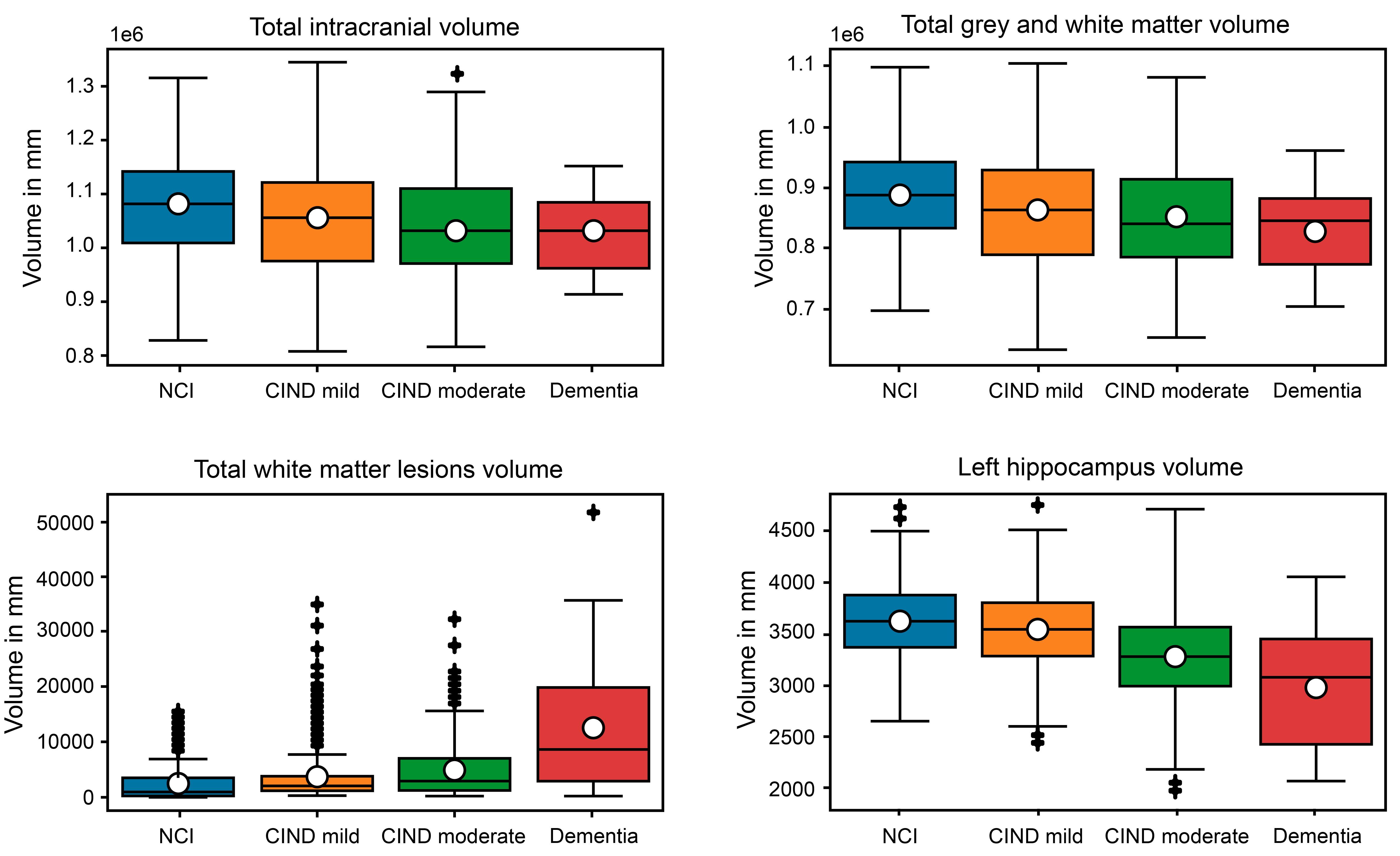 Table 3:
NCI vs. CIND Mild
NCI vs. CIND
ModerateNCI vs. Dementia
CIND Mild vs. CIND moderate
CIND Mild vs. Dementia
CIND Moderate vs. Dementia
ICV
0.0041
<0.0001
0.0084
0.1007
0.1057
0.4892
GWM
0.0016
<0.0001
0.0023
0.0873
0.1226
0.4330
WML
0.0029
<0.0001
0.0004
0.0005
0.0013
0.0084
LH
0.0181
<0.0001
<0.0001
<0.0001
<0.0001
0.0144
Table 4:
Feature
Category
NCI
CIND
MildCIND
ModerateDementia
Total
Prevalence
(in %)
No. of lacunes
0
223
216
200
13
652
65.80
>0
15
42
63
14
134
88.81
CMI numbers
0
232
247
243
20
742
68.73
>0
6
11
20
7
44
86.36
Central
atrophyrateNone
24
37
10
0
71
66.20
Mild
169
164
148
8
489
65.44
Moderate
42
51
90
15
189
78.39
Severe
2
6
15
4
27
92.59
No. of cortical infarcts
0
235
250
255
26
766
69.32
>0
3
8
8
1
20
85.00
No. of stenosed artery
0
216
226
221
18
681
68.28
>0
22
32
42
9
105
79.05
3.1. Overview of the Methods Used In this section, three classifiers, namely, multinomial logistic regression, XGBoost, and Autoencoder have been applied to a three-class classification task. The sample sizes for the three groups were 238, 258, and 290, respectively. The cleaned dataset was split into two parts: 80% was used for training and the remaining 20% was used for testing. The experiment was performed on Windows 10 Pro using Python (version 3.9.6) on a 2.3 GHz intel core i7, with 4 cores and 16 GB RAM. An overview of the research framework for our study is shown in Figure 2 below. 3.2. Multinominal Logistic Regression The Logistic Regression (LR) is a powerful supervised machine learning algorithm used for binary classification problems. The Multinomial Logistic Regression (MLR) [24], also known as softmax regression, is a classification method that extends the Logistic Regression to handle multiclass problems. It estimates the probability of each category relative to a reference category by applying the softmax function to a set of linear predictors, resulting in probabilities that sum to one. The model calculates log-odds ratios for each category in comparison to the reference category, with coefficients estimated through maximum likelihood estimation. Before building the MLR models, it is essential to ensure that the following two key assumptions have been satisfied: The independent variables should be independent of each other, meaning the model should have little or no multicollinearity. Only meaningful variables should be included in the model. Therefore, we first removed variables that were highly correlated, defining high correlation as an absolute value greater than 0.7. For example, since the volumes of the LH and RH were highly correlated, we removed the RH volume from the dataset. After eliminating these highly correlated variables, we normalized the cleaned dataset. For numeric variables, we applied Z-score normalization, and for categorical variables, we used label encoding, which converts each category value into a numerical label. The numerical labels range from 0 to the number of categories minus one. We used the training dataset to build the MLR model, initially including all variables. The optimal MLR model was determined manually by sequentially removing variables until all remaining regression coefficients were significantly different from 0 at the chosen alpha level of 0.05. This MLR analysis was performed using the Python library Scikit-learn [25,26]. 3.3. Extreme Gradient Boosting Extreme Gradient Boosting (XGBoost) is a scalable, end-to-end tree boosting system introduced in [26], designed to implement gradient boosted decision trees with a focus on speed and performance. It has recently become a dominant method in applied machine learning methods for tabular data. Instead of fitting a single large tree, XGBoost uses an ensemble of smaller trees, each built sequentially based on the residuals of the previous trees. Specifically, after adding a new tree, XGBoost adjusts the residuals of the previous model to correct errors and improve performance in areas where the model previously struggled. This approach helps reduce overfitting by using an ensemble of shallow trees rather than relying on a single large tree, which also aids in better generalization. In addition to its strong predictive capabilities, XGBoost allows for the evaluation of input variable importance. We implemented the XGBoost algorithm using the Python libraries Scikit-learn [25] and xgboost. The parameters in our experiment were set as follows: Subsample ratio of columns when constructing each tree: between 0 and 0.3 Minimum loss reduction required to make a further partition on a leaf node: between 0 and 0.5 Boosting learning rate: between 0.01 and 0.05 Maximum tree depth for base learners: integers between 1 and 4 Number of boosting rounds: integers between 200 and 500 Subsample ratio of the training instances: between 0.8 and 1 The hyperparameters were tuned using cross-validation. To prevent overfitting, early stopping was employed. The model stops if the score does not improve after 5 rounds. 3.4. Autoencoder An autoencoder is an unsupervised ANN algorithm that aims to produce output identical to its input. As outlined in Section 1, the architecture of an autoencoder is structured to learn efficient representations of the input data. When used for anomaly detection, setting a threshold for the reconstruction error is crucial but can be challenging and subjective as well. Therefore, to address this issue in the multiclass classification problem, we trained k autoencoder models in this study, one for each class, rather than training a single autoencoder model solely on normal observations. For example, there are three classes in this study, that is, NCI, CIND mild, and CIND moderate/Dementia. We therefore train three separate autoencoder models, each using data from one of the three classes. For any new observation, we compute three reconstruction errors by inputting it into the three trained autoencoder models, respectively. The new observation is then assigned to the class with the smallest reconstruction error. The architecture of the autoencoder is detailed as follows. The categorical variables were represented using one-hot encoding, and the entire dataset was normalized into range [−1, 1] using min-max normalization. The autoencoder models used in this study are structured with fully connected networks for both the encoder and decoder. Each autoencoder includes one fully connected hidden layer, with batch normalization [27]. The activation function of the decoder’s last layer is Tanh, while LeakyReLU [28] with a negative slope of 0.2 is used for the hidden layers. To prevent overfitting, dropout [29] is applied to each hidden layer. Mean Square Error (MSE) is used as the reconstruction error metric. The autoencoder was implemented using the Python deep learning library, PyTorch [30], and its detailed structure can be found in the source available online (31]. For all three autoencoders, the optimal models were configured with a hidden layer width of 24, an embedding space dimension of 12, and a batch size of 100. The learning rate is set to 0.005 for the NCI-autoencoder and CIND moderate/Dementia-autoencoder, while it is slightly higher at 0.008 for the CIND mild-autoencoder. The number of epochs is 700 for the NCI-autoencoder and CIND moderate/Dementia-autoencoder, and 600 for the CIND mild-autoencoder. The dropout rates for the three classifiers are set to 0.15, 0.1, and 0.2, respectively. Understanding the feature importance by analyzing the latent space of the trained autoencoder model is also crucial. This study proposes an intuitive method for estimating the feature importance based on the latent space representations learned by the trained autoencoder. Let the input data be represented as To estimate feature importance, the following procedure is followed after training the autoencoder. Firstly, we normalize the identity matrix Ip using the min-max normalization, scaling the entries of the identity matrix to the range of [−1, 1], and input it into the trained encoder. The identity matrix has ones on the diagonal and zeros elsewhere, which effectively “activates” each feature individually. Each column of Ip corresponds to one input feature being set to 1, while all other features are set to 0. The resulting encoded data corresponds to the latent space representation 
This subsection represents the results of the three-class classification problem using the proposed autoencoder algorithm alongside MLR and XGBoost. In the test dataset, which contains 158 observations, 45 are from the NCI class, 50 from the CIND mild class, and 63 from the CIND moderate/Dementia class. Various performance metrics, including overall accuracy, precision, recall, and F1-score, were used to evaluate the performance of MLR, XGBoost and the autoencoder. Except for overall accuracy, the other three metrics are used for binary classification and compute the relationship between the true positives (TP), true negatives (TN), false positives (FP), and false negatives (FN) classified by the model. The equations below show how to calculate these metrics for each class: Figure 3 below displays the confusion matrices provided by MLR, XGBoost and the autoencoder, with ‘0’ representing the NCI group, ‘1’ representing the CIND mild group, and ‘2’ representing the CIND moderate/Dementia group. The detailed values for overall accuracy, precision, recall, and F1_score are presented in Table 5. Classification results given by MLR, XGBoost and the Autoencoder. Several conclusions can be drawn from Figure 3 and Table 5. First, the autoencoder outperforms the other two machine learning methods in terms of overall accuracy and precision, achieving the highest accuracy at 0.6203, and the highest precision across all three groups. Notably, the proposed autoencoder classifier excels in classifying observations from the CIND mild group. As shown in Figure 3, the autoencoder achieves the best performance in correctly classifying the CIND mild group, while MLR and XGBoost only correctly classify 16 and 12 observations, respectively. In contrast, MLR and XGBoost more accurately classify observations from the CIND moderate/Dementia group, as seen from Figure 3, with 43 and 46 correctly classified observations, respectively. This is likely due to the clearer distinction between CIND moderate/Dementia and the other groups, such as CIND mild and NCI. However, the autoencoder classifier effectively differentiates between CIND mild and NCI, benefiting from its independent training on each class. This capability is crucial for accurately classifying cognitive impairment at various levels. Additionally, the autoencoder also achieved the highest F1-score for the NCI and CIND mild groups, and a comparable F1-score with the other two competitors for the CIND moderate/Dementia group. Based on the feature importance provided by these three classifiers, several insights can be gathered. Firstly, all three classifiers—MLR, XGBoost, and the autoencoder—consistently indicate that basic demographic information and neuroimaging markers are more important than the risk factors. Specifically, the final MLR model includes all four demographic variables and two neuroimaging markers (WML and LH). Among the top 10 features identified by XGBoost, two are demographic variables (Age and Education Level), seven are neuroimaging markers, and another one is BMI. The feature importance derived from the autoencoder aligns well with those from MLR and XGBoost, highlighting the significance of the four demographic variables in detecting cognitive impairments. Additionally, beyond WML and LH, the autoencoder also highlights the importance of the number of cortical infarcts and the number of stenosed arteries. These results are consistent with the exploratory data analysis, presented in Section 2.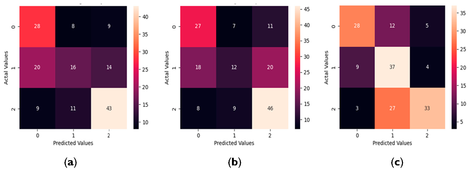 Table 5:
MLR
XGBoost
Autoencoder
Precision
Recall
F1
Precision
Recall
F1
Precision
Recall
F1
NCI
0.49
0.62
0.55
0.51
0.60
0.55
0.70
0.62
0.66
CIND mild
0.46
0.32
0.38
0.43
0.24
0.31
0.49
0.74
0.59
CIND moderate/Dementia
0.65
0.68
0.67
0.60
0.73
0.66
0.79
0.52
0.63
Overall Accuracy
0.5506
0.5380
0.6203
In this study, a deep learning autoencoder algorithm was utilized in combination with two machine learning classifiers, namely MLR and XGBoost, to predict cognitive impairment using data from a study conducted in Singapore. A novel approach has been propsoed that leverages the autoencoder for multiclass classification problems, eliminating the need to determine a threshold for reconstruction errors. The classification results demonstrate that the autoencoder outperforms the other two classifiers in terms of overall accuracy and excels particularly in classifying observations from the CIND mild group. Additionally, we introduced a new method for deriving feature importance from the autoencoder classifier, which aligns well with the feature importance identified by MLR and XGBoost. The results indicate that basic demographic information and neuroimaging markers are more crucial than risk factors. The EDIS study collected participant information through questionnaires, physical examinations, and laboratory tests. The findings from this study could inform the redesign of the questionnaire to make it more concise and accurate. Additionally, reducing the number of domains tested in the NTB assessment, which takes about an hour per person, could save significant time and resources. Further research in this direction, including comprehensive brain region segmentation and the selection of critical regions using advanced methods, is warranted. The method is straightforward, and the necessary features are easy to collect. However, the limitations of the dataset affected classification accuracy and the comprehensiveness of predicting cognitive impairment using neuroimaging markers. The dataset includes only the total volumes of ICV, GWM, WML, GM, WM, LH, RH, and cerebrospinal fluid, many of which are highly correlated and may not fully capture the complexity of brain MRI information. Image segmentation to obtain volumes of all brain regions is necessary. Identifying significant regions for predicting cognitive impairment using machine learning and deep learning methods is an area of future interest. Additionally, it would be valuable to compare our proposed classifier with deep learning methods discussed in Section 1, such as CNNs, in future work.
Conceptualization and supervision, T.Z., C.A.H., Y.X.C., C.C.L.-H. and S.H.; methodology, T.Z., C.A.H. and Y.X.C.; validation, T.Z., C.A.H. and Y.X.C.; formal analysis, T.Z. and Y.X.C.; investigation, T.Z., C.A.H. and Y.X.C.; resources, S.H.; data curation, C.C.L.-H.; writing—original draft preparation, T.Z. and Y.X.C.; writing—review and editing, T.Z., C.A.H. and Y.X.C.; project administration, C.A.H. All authors have read and agreed to the published version of the manuscript.
Data supporting the results of this study are available upon request.
Not applicable.
The authors declare no conflicts of interest regarding this manuscript.
No external funding was received for this research.
The authors would like to thank the reviewers for their time, effort, and thoughtful comments and suggestions which help improve the paper substantially.
[1] E.B. Larson, K.M. Langa, "The rising tide of dementia worldwide" Lancet, vol. 372, no. 9637, pp. 430-432, 2008. [Crossref]
[2] , "Global dementia cases forecasted to triple by 2050," in The Alzheimer’s Association International Conference, Jul. 26–30, 2021, virtual, pp. -.
[3] S. Savaş, "Detecting the stages of Alzheimer’s disease with pre-trained deep learning architectures" Arab. J. Sci. Eng., vol. 47, no. 2, pp. 2201-2218, 2022. [Crossref]
[4] A. Krizhevsky, I. Sutskever, G.E. Hinton, "Imagenet classification with deep convolutional neural networks" Adv. Neural Inf. Process. Syst., vol. 25, 2012. [Crossref]
[5] N.T. Duc, S. Ryu, M.N.I. Qureshi, M. Choi, K.H. Lee, B. Lee, "3D-deep learning based automatic diagnosis of Alzheimer’s disease with joint MMSE prediction using resting-state fMRI" Neuroinformatics, vol. 18, pp. 71-86, 2020. [Crossref] [PubMed]
[6] S. Murugan, C. Venkatesan, M.G. Sumithra, X.Z. Gao, B. Elakkiya, M. Akila, "DEMNET: A deep learning model for early diagnosis of Alzheimer diseases and dementia from MR images" IEEE Access, vol. 9, pp. 90319-90329, 2021. [Crossref]
[7] F.J.M. Shamrat, S. Akter, S. Azam, A. Karim, P. Ghosh, Z. Tasnim, "AlzheimerNet: An effective deep learning based proposition for alzheimer’s disease stages classification from functional brain changes in magnetic resonance images" IEEE Access, vol. 11, pp. 16376-16395, 2023. [Crossref]
[8] F. Ramzan, M.U.G. Khan, A. Rehmat, S. Iqbal, T. Saba, A. Rehman, "A deep learning approach for automated diagnosis and multi-class classification of Alzheimer’s disease stages using resting-state fMRI and residual neural networks" J. Med. Syst., vol. 44, pp. 1-16, 2020. [Crossref]
[9] K. Oh, Y.-C. Chung, K.W. Kim, W.-S. Kim, I.-S. Oh, "Classification and visualization of Alzheimer’s disease using volumetric convolutional neural network and transfer learning" Sci. Rep., vol. 9, no. 1, 2019. [Crossref]
[10] C. Dachena, S. Casu, M.B. Lodi, A. Fanti, G. Mazzarella, "Application of MRI, fMRI and cognitive data for Alzheimer’s disease detection," in 2020 14th European conference on antennas and propagation (EuCAP), , Eds. New York, NY, USA: IEEE, 2020, pp. 1-4.
[11] M.J. Kang, S.Y. Kim, D.L. Na, B.C. Kim, D.W. Yang, E.J. Kim, "Prediction of cognitive impairment via deep learning trained with multi-center neuropsychological test data" BMC Med. Inform. Decis. Mak., vol. 19, pp. 1-9, 2019. [Crossref]
[12] D. Aschwanden, S. Aichele, P. Ghisletta, A. Terracciano, M. Kliegel, A.R. Sutin, "Predicting cognitive impairment and dementia: A machine learning approach" J. Alzheimer’s Dis., vol. 75, no. 3, pp. 717-728, 2020. [Crossref]
[13] C. Lian, M. Liu, L. Wang, D. Shen, "Multi-task weakly-supervised attention network for dementia status estimation with structural MRI" IEEE Trans. Neural Netw. Learn. Syst., vol. 33, no. 8, pp. 4056-4068, 2021. [Crossref] [PubMed]
[14] V. Jain, O. Nankar, D.J. Jerrish, S. Gite, S. Patil, K. Kotecha, "A novel AI-based system for detection and severity prediction of dementia using MRI" IEEE Access, vol. 9, pp. 154324-154346, 2021. [Crossref]
[15] P. Gajjar, M. Garg, S. Desai, H. Chhinkaniwala, H.A. Sanghvi, R.H. Patel, "An Empirical Analysis of Diffusion, Autoencoders, and Adversarial Deep Learning Models for Predicting Dementia Using High-Fidelity MRI" IEEE Access, vol. 12, pp. 131231-131243, 2024. [Crossref]
[16] K.J. Holyoak, "Parallel distributed processing: explorations in the microstructure of cognition" Science, vol. 236, pp. 992-997, 1987. [Crossref] [PubMed]
[17] C. Baur, S. Denner, B. Wiestler, N. Navab, S. Albarqouni, "Autoencoders for unsupervised anomaly segmentation in brain MR images: a comparative study" Med. Image Anal., vol. 69, p. 101952, 2021. [Crossref]
[18] A. Paszke, S. Gross, F. Massa, A. Lerer, J. Bradbury, G. Chanan, "Prevalence of cognitive impairment in Chinese: epidemiology of dementia in Singapore study" J. Neurol. Neurosurg. Psychiatry, vol. 84, no. 6, pp. 686-692, 2013. [Crossref] [PubMed]
[19] S. Hilal, C.S. Tan, X. Xin, S.M. Amin, T.Y. Wong, C. Chen, "Prevalence of cognitive impairment and dementia in Malays-epidemiology of dementia in Singapore study" Curr. Alzheimer Res., vol. 14, no. 6, pp. 620-627, 2017. [Crossref]
[20] M.Y.Z. Wong, C.S. Tan, N. Venketasubramanian, C. Chen, M.K. Ikram, C.Y. Cheng, "Prevalence and risk factors for cognitive impairment and dementia in Indians: a Multiethnic Perspective from a Singaporean Study" J. Alzheimer’s Dis., vol. 71, no. 1, pp. 341-351, 2019. [Crossref]
[21] D. Yeo, C. Gabriel, C. Chen, S. Lee, T. Loenneker, M. Wong, "Pilot validation of a customized neuropsychological battery in elderly Singaporeans" Neurol. J. South East Asia, vol. 2, no. 123, 1997.
[22] , "The probable error of a mean" Biometrika, pp. 1-25, 1908.
[23] M.S. Bartlett, "Properties of sufficiency and statistical tests" Proc. R. Soc. London. Ser. A-Math. Phys. Sci., vol. 160, no. 901, pp. 268-282, 1937. [Crossref]
[24] D. Böhning, "Multinomial logistic regression algorithm" Ann. Inst. Stat. Math., vol. 44, no. 1, pp. 197-200, 1992. [Crossref]
[25] F. Pedregosa, G. Varoquaux, A. Gramfort, V. Michel, B. Thirion, O. Grisel, "Scikit-learn: Machine learning in Python" J. Mach. Learn. Res., vol. 12, pp. 2825-2830, 2011. [Crossref]
[26] T. Chen, C. Guestrin, "Xgboost: A scalable tree boosting system," in Proceedings of the 22nd acm sigkdd international conference on knowledge discovery and data mining, Aug. 13–17, 2016, San Francisco, CA, USA, pp. 785-794.
[27] S. Ioffe, C. Szegedy, "Batch normalization: Accelerating deep network training by reducing internal covariate shift," in International conference on machine learning, Jul. 6–11, 2015, Lille, France, pp. 448-456.
[28] A.L. Maas, A.Y. Hannun, A.Y. Ng, "Rectifier nonlinearities improve neural network acoustic models," in Proceedings of the 30th International Conference on International Conference on Machine Learning, Jun. 16–21, 2013, Atlanta, GA, USA, pp. 3-.
[29] N. Srivastava, G. Hinton, A. Krizhevsky, I. Sutskever, R. Salakhutdinov, "Dropout: a simple way to prevent neural networks from overfitting" J. Mach. Learn. Res., vol. 15, no. 1, pp. 1929-1958, 2014. Available online: https://jmlr.org/papers/v15/srivastava14a.html.
[30] A. Paszke, S. Gross, F. Massa, A. Lerer, J. Bradbury, G. Chanan, "PyTorch: An Imperative Style, High-Performance Deep Learning Library," in presented at the Advances in Neural Information Processing Systems 32, Dec. 8–14, 2019, Vancouver, BC, Canada, pp. -.
[31] T. Akiba, S. Sano, T. Yanase, T. Ohta, M. Koyama, "Optuna: A Next-generation Hyperparameter Optimization Framework," in Proceedings of the 25th ACM SIGKDD international conference on knowledge discovery & data mining, Aug. 4–8, 2019, Anchorage, AK, USA, pp. 2623-2631.